Source From: https://15445.courses.cs.cmu.edu/fall2020/schedule.html
Hash Tables
Data Structures
A DBMS uses various data structures for many different parts of the system internals. Some examples include:
- Internal Meta-Data: This is data that keeps track of information about the database and the system state. Ex: Page tables, page directories.
- Core Data Storage: Data structures are used as the base storage for tuples in the databse.
- Temporary Data Structures: The DBMS can build data structures on the fly while processing a query to speed up execution (e.g. hash tables for joins).
- Table indices: Auxiliary(辅助的) data structures can be used to make it easier to find specific tuples.
There are two main design decisions to consider when implementing data structures for the DBMS:
- Data organization: We need to figure out how to layout memory and what information to store inside the data structure in order to support the efficient access.
- Concurrency: We also need to think about how to enable multiple therads to access the data structure without causing problems.
Hash Table
A hash table implements an associative array abstract data type that maps keys to values. It provides on average O(1) operation complexity (O(n) is the worst-case) and O(n) storage complexity. Note that even with O(1) operation complexity on average, there are constant factor optimizations which are important to consider in the real world.
A hash table implementation is comprised of two parts
- Hash Function: This tells us how to map a large key space into a smaller domain. It is used to compute an index into an array of buckets or slots. We need to consider the trade-off between fast execution and collision rate. On one extreme, we have a hash function that always returns a constant (very fast, but everything is a collision). On the other extreme, we have a “perfect” hashing function where there are no collisions, but would take extremely long to compute. The ideal design is somewhere in the middle.
- Hashing Scheme: This tells us how to handle key collisions after hashing. Here, we need to consider the trade-off between allocating a large hash table to reduce collisions and having to execute additional instructions when a collision occurs.
Hash Functions
A hash function takes in any key as its input. It then returns an integer representation of that key (i.e. the “hash”). The function’s output is deterministic (i.e. the same key should always generate the same hash output).
The DBMS need not use a cryptographically(加密的) secure hash function (e.g., SHA-256) because we do not need to worry about protecting the contents of keys. These hash functions are primarily used internally by the DBMS and thus information is not leaked outside of the system. In general, we only care about the hash function’s speed and collision rate.
The current state-of-the-art hash function is Facebook XXHash3.
Static Hashing Schemes
A static hashing scheme is one where the size of the hash table is fixed. This means that if the DBMS runs out of storage space in the hash table, then it has to rebuild a larger hash table from scratch, which is very expensive. Typically the new hash table is twice the size of the original hash table.
To reduce the number of wasteful comparisons, it is important to avoid collisions of hashed key. Typically, we use twice the number of slots as the number of expected elements.
The following assumptions usually do not hold in reality:
- The number of elements is known ahead of time.
- Keys are unique.
- There exists a perfect hash function.
Therefore, we need to choose the hash function and hashing scheme appropriately.
Linear Probe Hashing
This is the most basic hashing scheme. It is also typically the fastest. It uses a circular buffer of array slots. The hash function maps keys to slots. When a collision occurs, we linearly search the adjacent slots until an open one is found. For lookups, we can check the slot the key hashes to, and search linearly until we find the desired entry (or an empty slot, in which case the key is not in the table). Note that this means we have to store the key in the slot as well so that we can check if an entry is the derired one.

Deletions are more tricky. We have to be careful about just removing the entry from the slot, as this may prevent future lookups from the finding entries that have been put below the now empty slot. There are two solutions to this problem:
- The most common approach is to use “tombstones”. Instead of deleting the entry, we replace it with a “tombstone” which tells future lookups to keep scanning.
- The other option is to shift the adjacent data after deleting an entry to fill the now empty slot. However, we must be careful to only move the entries which were originally shifted.


Non-unique Keys: In the case where the same key may be associated with multiple different values or tuples, there are two approaches.
- Seperate Linked List: Instead of sorting the values with the keys, we store a pointer to a seperate storage area which contains a linked list of all the values.
- Redundant Keys: The more common approach is to simply store the same key multiple times in the table. Everything with linear probing still works even if we do this.

Robin Hood Hashing
This is an extension of linear probe hashing that seeks to reduce the maximum distance of each key from their optimal position (i.e. the original slot they were hashed to) in the hash table. This strategy steals slots from “rich” keys and gives them to “poor” keys.
In this variant, each entry also records the “distance” they are from their optimal position. Then, on each insert, if the key being inserted would be farther away from their optimal position at the current slot than the current entry’s distance, we replace the current entry and continue trying to insert the old entry farther down the table.
Cuckoo Hashing
Instead of using a single hash table, this approach maintains multiple has tables with different hash functions. The hash functions are the same algorithm (e.g. XXHash, CityHash); they generate different hashes for the same key by using seed values.
When we insert, we check every table and choose one that has a free slot (if multiple have one, we can compare things like load factor, or more commonly, just choose a random table). If no table has a free slot, we choose (typically a random one) and evict the old entry. We then rehash the old entry into a different table. In rare cases, we may end up in a cycle. If this happens, we can rebuild all of the hash tables with new hash function seeds (less common) or rebuild the hash tables using larger tables (more common).
Cuckoo hashing guarantees O(1) lookups and deletions, but insertions may be more expensive.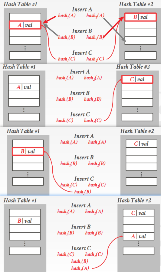
Dynamic Hashing Schemes
The static hashing schemes require the DBMS to know the number of elements it wants to store. Otherwise, it has to rebuild the table if it needs to grow/shrink in size.
Dynamic hashing schemes are able to resize the hash table on demand without needing to rebuild the entire table. The schemes perform this resizing in different ways that can either maximize reads ot writes.
Chained Hashing
This is the most common dynamic hashing scheme. The DBMS maintains a linked list of buckets for each slot in the hash table. Keys which hash to the same slot are simply inserted into the linked list for that slot.
Extendible Hashing
Improved variant of chained hashing that splits buckets instead of letting chains to grow forever. This approach allows multiple slot locations in the hash table to point to the same bucket chain.
The core idea behind re-balancing the hash table is to move bucket entries on split and increase the number of bits to examine to find entries in the hash table. This means that the DBMS only has to move data within the buckets of the split chain; all other buckets are left untouched.
- The DBMS maintains a global and local depth bit counts that determine the number bits needed to find buckets in the slot array.
- When a bucket is full, the DBMS splits the bucket and reshuffle its elements. If the local depth of the split bucket is less than the global depth, then the new bucket is just added to the exiting slot array. Otherwise, the DBMS doubles the size of the slot array to accommodate the new bucket and increments the global depth counter.

Linear Hashing
Instead of immediately splitting a bucket when it overflows, this scheme maintains a split pointer that keeps track of the next bucket to split. No matter whether this pointer is pointing to a bucket that overflowed, the DBMS always splits. The overflow criterion is left up to the implementation.
- When any bucket overflows, split the bucket at the pointer location by adding a new slot entry, and create a new hash function.
- If the hash function maps to slot that has previously been pointed to by pointer, apply the new hash function.
- When the pointer reaches last slot, delete original hash function and replace it with a new hash function.

- 本文作者: 夏花
- 本文链接: http://xiahua19.github.io/2022/08/30/cmu15-5-Hash-Tables/
- 版权声明: 本博客所有文章除特别声明外,均采用 MIT 许可协议。转载请注明出处!